

Overview
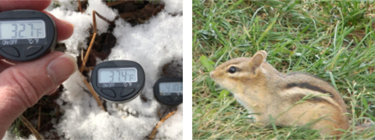
How do animals survive the winter in cold climates? Many hibernate underground – but why is the underground environment warmer than the surface? The answer is sunlight stored in soil. With very simple tools we can explore the shallow subsurface environment and learn a lot more about how natural and human communities benefit from sunlight stored in soil.
Introduction
Students measure a soil temperature profile to explore the effect of energy from the Sun on the shallow subsurface environment. Multiple temperature profiles allow students to analyze the daily change in energy that diffuses into the subsurface, and its differential impact near the surface and at depth.
Grade Level
6-8, 9-12
At the middle school level, you might want to graph only the spatial change in temperature, and relate these data to the ability of organisms to hibernate underground through winter. At the high school level, graph data in both spatial and temporal coordinates. Relate the results to both natural and human communities.
Learning Objectives
Students will
- practice recording and graphing data
- analyze and interpret their graphed results
- extend their results to consider the impact of solar thermal energy on natural ecosystems and consider the energy opportunities for human communities.
Lesson Format
In School: This is a lab/field activity. Outdoor measurements are ideal, but the experiment can be set up in an indoor setting such as a terrarium or flower pot. Students will graph the data they record, which can be done by hand on the supplied graph paper, or can be done on a computer with appropriate software.
Virtual Lab: This activity can be done in a remote learning environment where students watch the experiment on video and work with the resulting data.
Time Required
This activity is more interesting the more time you can devote to it. It is possible to measure, graph, and discuss a single soil temperature profile in a single class period. If you have the ability to make multiple measurements over the course of the day (e.g. with different class sections), or make measurements in different seasons, the resulting data give a much richer picture of energy stored in the shallow subsurface, and the way it changes with time of day and with the changing seasons.
Standards
NGSS:
Analyzing & Interpreting Data
PS3.D Energy in everyday life
ESS3.D Global climate change
Energy & Matter
Credits & Contact Info
Dr. Alexandra Moore
Paleontological Research Institution, 1259 Trumansburg Rd., Ithaca NY 14850
moore@priweb.org
Instructions & Materials
Resources
- Video | In the Greenhouse #7 | Sunlight Stored in Soil
- Virtual Lab Video
- Instructor Handout (pdf, 4.3 MB)
- Student Handout (pdf, 2.9 MB)
- Data spreadsheet: Soil Temperature Profiles (xlsx, 285 kb)
In-School Activity
- Download the Instructor Handout, Student Handout, and Data Spreadsheet.
The Instructor Handout duplicates all the content of the Student Handout, with additional context and directions for setting up and running the experiment. The data spreadsheet contains several different datasets, including high-resolution soil temperature profiles from a temperate latitude site in upstate New York, and a full years of once-daily data from a nearby NOAA monitoring station.
- Set up and run the experiment yourself first, to gauge the range of temperatures your students are likely to encounter in your particular environment and season. Decide how best to have students set up axes on their graphs based on the range of temperatures you have observed.
Materials
One set of materials for each group of 2 - 5 students:
- Soil-filled terrarium, flowerpot – OR – appropriate outdoor field site
- 6” metal-stem digital thermometers (2 or 3 per group, depending on experimental design). Kitchen thermometers work just as well as actual soil thermometers.
- Clip lamp w/ high intensity bulb (if indoors)
- Student lab handout (1 per student)
- Optional: a steel knitting needle can be helpful when inserting the thermometers into outdoor soil - use the needle to make a guide hole for the thermometer so that it slides in and out of the soil without damage
Virtual Activity
This activity can be completed as a virtual lab by watching the accompanying YouTube video and downloading the Soil Temperature Profiles spreadsheet.
-
Separate handout for virtual activity (pdf, 2.9 MB)
-
Virtual Lab video (see above)
Background & Extensions
Why?
One hundred seventy-four thousand terajoules (10¹² joules) of solar energy strike the surface of the Earth every second. This greatly exceeds every other energy source available to Earth. For example, Earthʻs internal energy – the power behind earthquakes and volcanoes – flows across the surface at only 44 terajoules per second. Some of the incoming solar energy is absorbed by Earth surface materials, warming them, before eventually re-radiating back to space. The warm subsurface of the solid Earth and ocean is a critical component of all of Earth’s ecosystems.
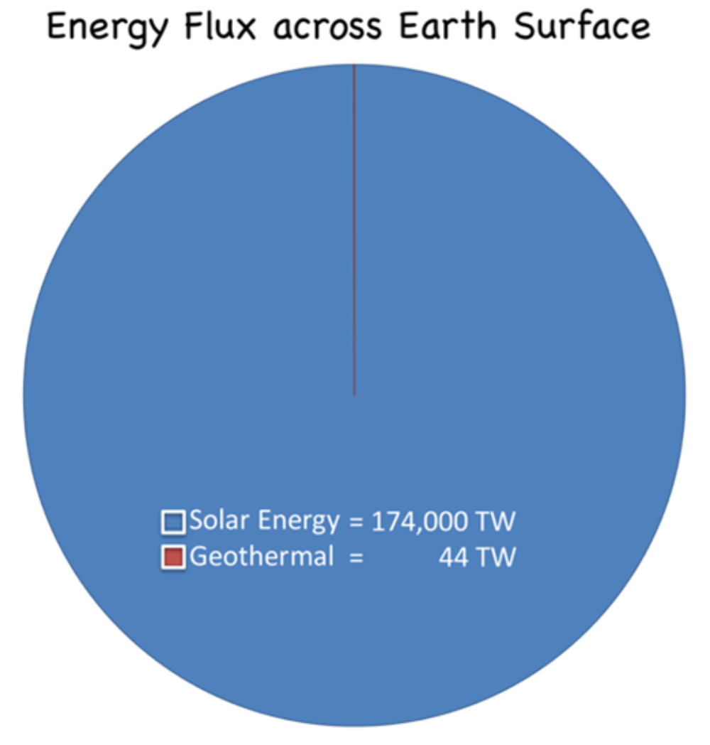
Figure 1: Pie chart comparison of solar geothermal energy flux across Earth’s surface.
What?
Incoming solar energy diffuses from the surface downward, creating a temperature gradient that we can measure. Because sunlight varies both seasonally and diurnally the temperature gradient is not constant, and it is not linear.
An easily accessible place to measure & examine the subsurface temperature gradient is in soil. We can graph our measured data to better understand the flux of energy through the subsurface, and to explore how natural and human communities can take advantage of this energy source.
Data Collection
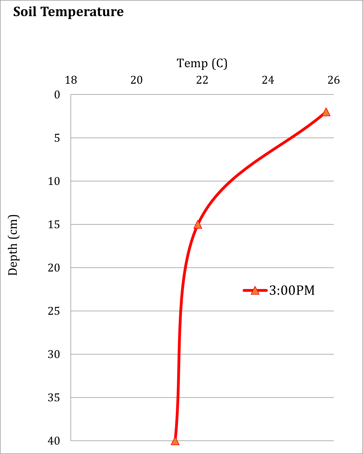
This experiment can be as simple as measuring two soil temperatures and then graphing the two data points. It can be as complicated as installing thermometers at multiple depths and leaving them in place to collect data for the entire school year. Or anything in between. The more data we collect the more interesting this experiment becomes. If we record the soil temperatures just once (for example, if we run the experiment indoors with artificial light in a single class period) we can compile a soil temperature profile for the time we made our measurements. A typical 3-point profile to a depth of 40 cm (16”) is shown in Figure 2.
Notice that for this graph, depth is plotted on the vertical axis, and that the values increase downward. This arrangement is unusual in two ways. First, y-axis values usually increase upward, and second, the dependent variable (temperature) is plotted here on the horizontal axis. These choices have been made because these data represent an actual physical space, thus the graph layout reflects that physical space as well.
Notice also that the temperature does not change as a linear function of depth. We are often tempted to draw straight lines through data – and we could make a “best fit” line here – but in this case the physical process that controls temperature at depth is not linear. The soil temperature is periodically changed by the daily appearance of the Sun (or lamp), thus the surface temperature is very dynamic, but the diffusion of the heat through the soil is slow, creating a curved temperature profile.
Figure 2: Soil temperature 0-40 cm, August, Ithaca, NY
If we repeat our measurements across the course of a school day we can make two graphs; one showing the spatial change of temperature in the soil and a second graph showing the temporal variation of temperature at each depth (Figure 3a).
Figure 3a: (Left) Summer soil temperature profiles from Ithaca NY at 9:00am, 12:00pm and 3:00pm. The 3pm data are the same as Figure 2. (Right) The same measurements plotted as a time series of soil temperatures at 2cm, 15cm, 40cm, from 9:00am to midnight.
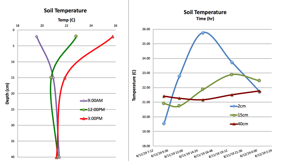
The first graph (left) shows the effect of daily heating and cooling of the Earth surface by sunlight. The first measurement of the day, at 9:00am, shows that the surface has not yet warmed up, and in fact the shallowest thermometer records the coolest temperature in the soil profile. Three hours later at 12:00 pm the surface has warmed somewhat – but notice the change at 15 cm depth. Here the soil is still “feeling” the coolness of the evening diffusing downward, and the temperature has decreased slightly, even as the shallow temperature increases. By 3:00 pm the surface is quite warm, and the warmth is moving downward through the soil, but does not yet affect the deepest thermometer at 40 cm (in fact the evening coolness has just now arrived at 40 cm, depressing the temperature a tiny amount).
The second graph (right) shows how heating and cooling vary as a function of time. Because the shallowest thermometer is closest to the source of heat it responds first and the magnitude of change is largest. As the heat diffuses downward the 15 cm thermometer responds, with a phase lag that follows the appearance of the Sun. The temperature here never gets as warm as the surface temperature because there isnʻt enough time; the soil at 15 cm is still warming up when the Sun sets and the surface begins to cool again. These two phenomena – the phase lag and a reduced amplitude of variation – are characteristic of processes controlled by diffusion. The deepest thermometer at 40 cm shows these effects even more strongly. The phase lag is longer, and the magnitude of change is very small. In fact, notice that the temperature at 40cm is warmest in the middle of the night!
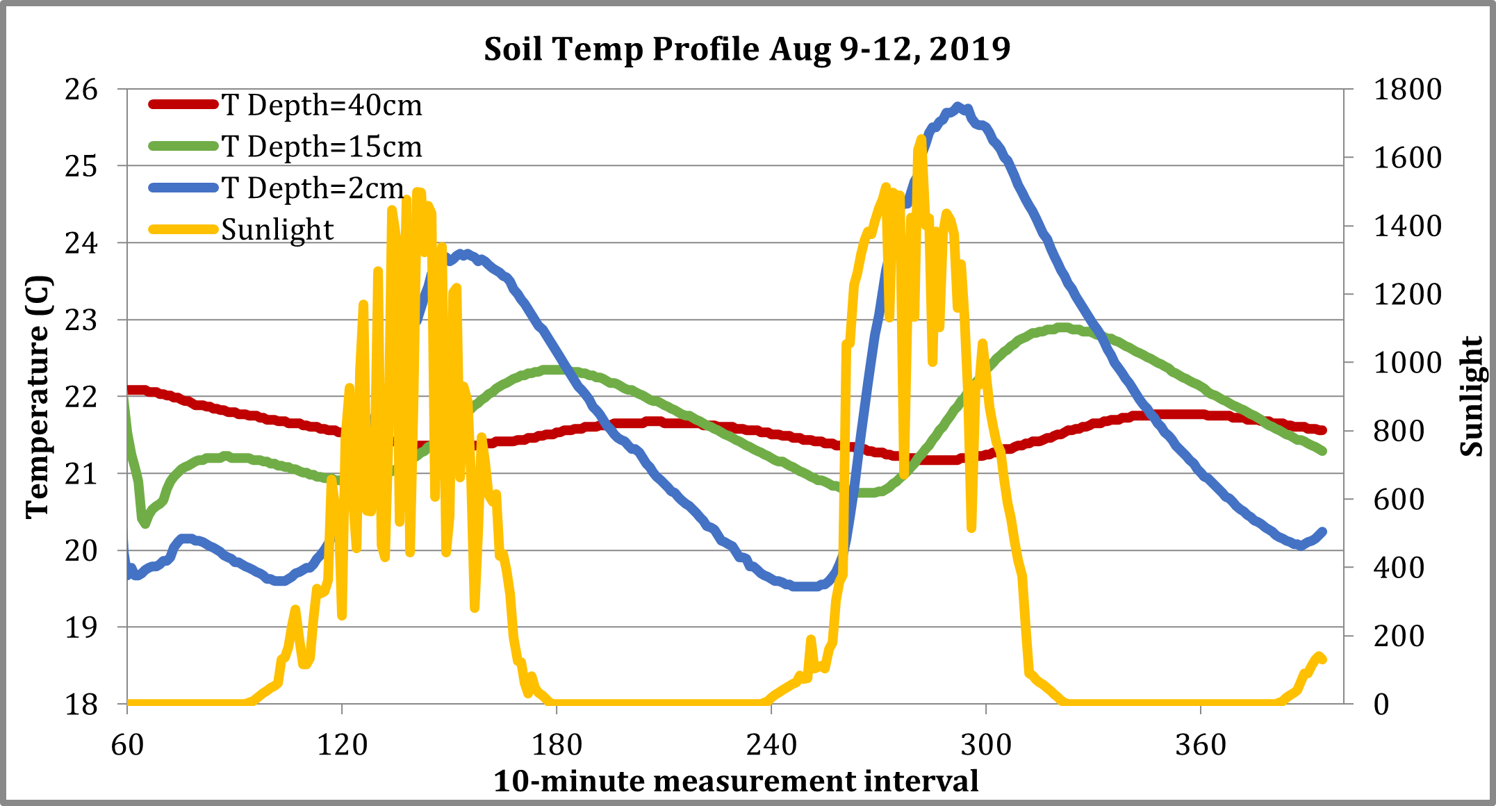
Figure 3b: Sunlight drives change in soil temperature. Two days of data with sunlight measurements (expanded data set from Figure 3a). The additional data shows the phase lag between the solar forcing and temperature at each depth even more clearly.
Seasonal Variation: How to stay warm in winter and cool in summer
Figure 4: Three months of soil temperature data at 2 cm and 40 cm, Ithaca, NY.
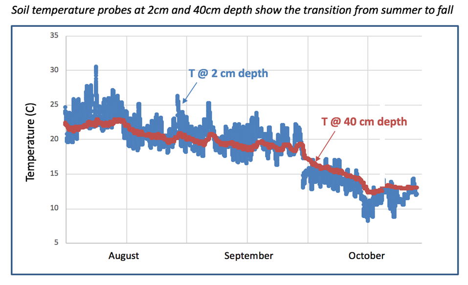
Just as the Sun changes the soil temperature on a daily basis, the seasonal change in sunlight intensity changes soil temperature over the course of the year. As with the daily variation that we observed above, the seasonal surface changes are largest, and the temperature change becomes smaller with increasing depth. In fact at temperate latitudes, there is very little change at all below a depth of about 3 meters (10 ft); the soil maintains a temperature equal to the annual average air temperature (ex: 55.7 F in Washington DC).
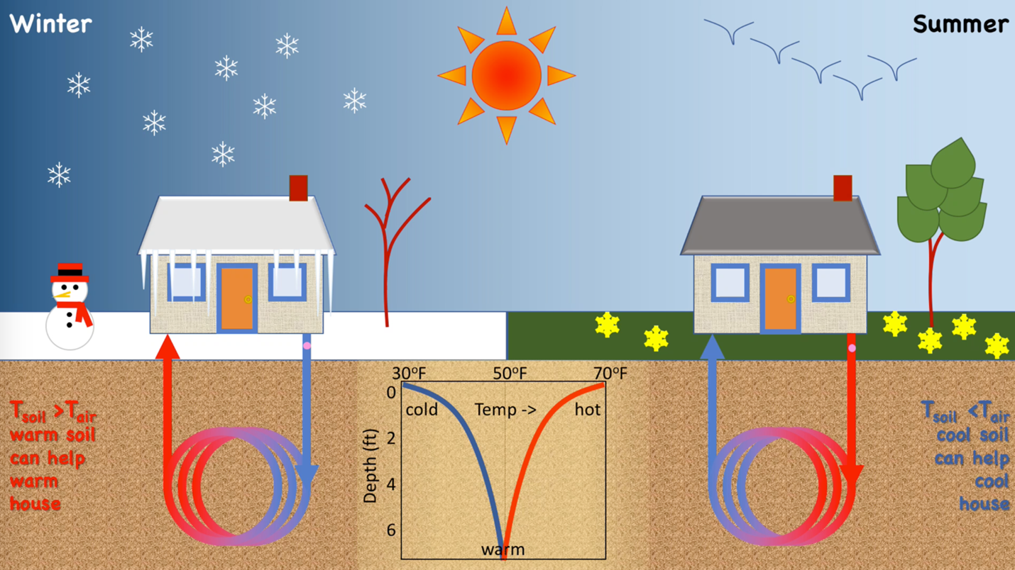
In Figure 4 we can see the transition from summer to fall in the soil temperature data. The surface temperature variation is always larger than the variation at a depth of 40 cm, but in the summer the near-surface soil is most often warmer than the deeper soil. As the seasons advance the surface soil becomes cooler than the deeper soil. At latitudes where the average annual air temperature is above freezing, the subsurface does not freeze. This is incredibly important for living organisms that need to hibernate through the winter. It is also very useful for human communities trying to keep warm in the cold months. Ground-sourced geothermal heat systems (Figure 5) take advantage of sunlight stored as heat in soil to warm residential and commercial buildings far more efficiently than conventional fossil-fuel powered heating systems. And ground-sourced heat pumps also work to cool buildings in the summer, when subsurface temperatures are reliably cooler than the air.
Figure 5: Diagram of a ground-source geothermal system. A pump circulates fluid through tubing buried in the ground. In winter the warm subsurface keeps the fluid warmer than the air, allowing for much more efficient heating of buildings. In summer the subsurface is cooler than air, cooling the circulating fluid for use in extremely energy-efficient air conditioning.
Examples
Campus-wide ground-source heat pump system at Ball State University, Indiana: https://www.bsu.edu/about/geothermal
Campus-wide lake source cooling system at Cornell University, New York: https://fcs.cornell.edu/departments/energy-sustainability/utilities/cooling-home/cooling-production-home/lake-source-cooling
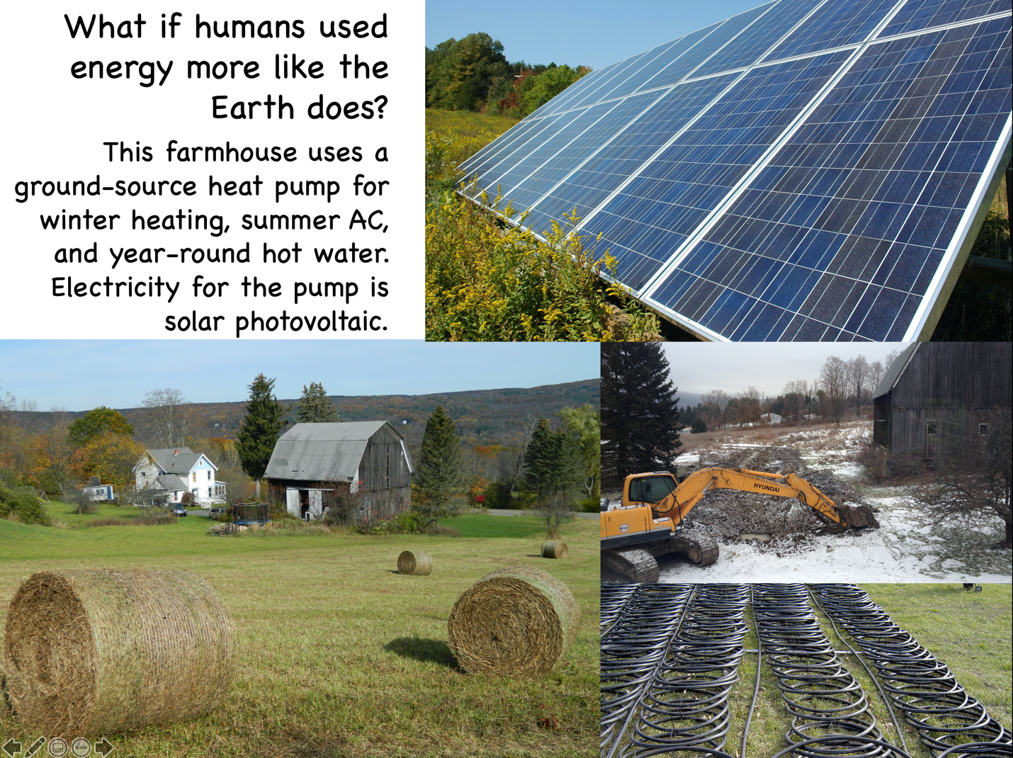
Figure 6: A farmhouse near Ithaca, NY, with installed solar photovoltaic and ground-source geothermal systems. Lower right photos show installation of the heat pumpʻs closed-loop tubing in trenches in front of the barn. The temperature of the fluid in the tubing is controlled by the soil, and maintains a year-round temperature of ~52F.
To better appreciate the efficiencies of ground-source geothermal energy, have students measure the air temperature when they make their soil temperature measurements. Air temperatures show large day-to-night and day-to-day variability, and by contrast, illustrate the stability of shallow subsurface temperatures.
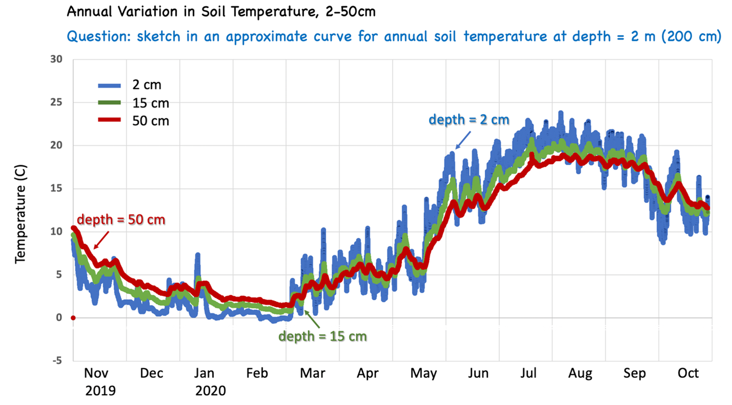
Figure 7: Twelve months of soil temperature data at the Cayuga Nature Center, Ithaca, NY.
Data from stations in every state are available for download in tabular text format. Note, however, that these data are not ready-to-use, and require some spreadsheet skills to format and graph. Also, the full records are *very large* files with lots of data, although there are different options to acquire subsets of the data.