

Overview
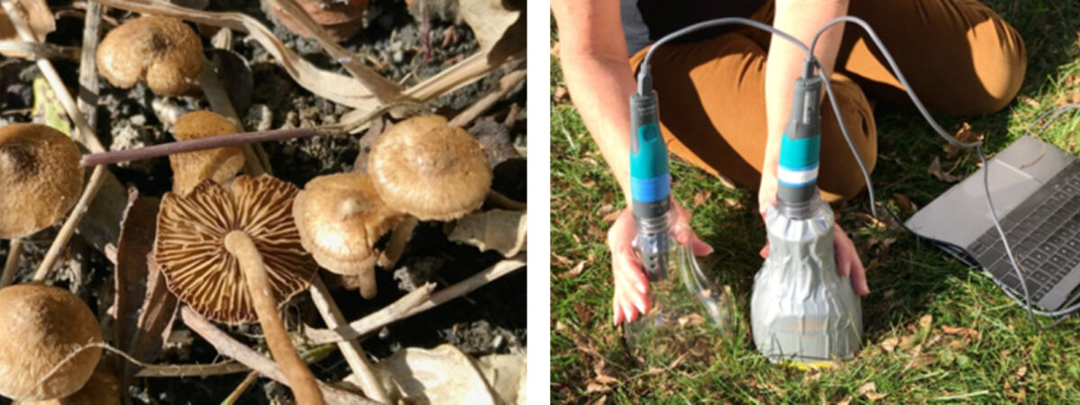
The forest recycles. In autumn when leaves fall bacteria, fungi, and other decomposers break down the carbohydrates created by photosynthesis, returning nutrients to the soil and CO₂ to the atmosphere. Respiration is part of the global carbon cycle, and represents a very large flux of carbon from biomass to the atmosphere; 120 gigatons of carbon annually. This flux is exactly balanced by photosynthesis – at least it is in natural systems. Humans upset the balance, pumping an additional 9 gigatons of carbon into the atmosphere every year. Quantifying the different carbon fluxes is important for understanding the carbon cycle and the changes in atmospheric chemistry and terrestrial ecosystems that are caused by humans.
Introduction
Students measure the flux of carbon dioxide from soil to the atmosphere using a lab CO₂ probe and home-made flux chambers. Despite the ad-hoc appearance of the experimental set-up the results are robust, and allow students to extend their analyses beyond the tiny plot of land that they directly observe. The experiment can be designed to allow students to manipulate the experimental conditions, and explore the relationship between temperature and respiration, pointing to an important consequence of global climate change. Simple graphing and applying a linear fit to the data incorporate numeracy skills in this activity.
Grade Level
6-8, 9-12
This activity is designed for high school students, but can be done in a less-quantitative way by middle school students. To complete the full set of data analyses covered here students will need to understand the concept of the mole as a measure of molecular mass.
Learning Objectives
Students will
- set up and conduct a CO₂ flux experiment
- practice recording and graphing data & plotting a linear best fit
- analyze and interpret their graphed results
- extend their results to consider the respiration flux of CO₂ beyond the study area, and place their observations within the context of the global carbon cycle
Lesson Format
In School: This is a lab/field activity that can be done indoors or outdoors. The advantage to working outdoors is that students measure actual environmental carbon fluxes. The indoor experiment has the advantage of being able to manipulate the experimental conditions - for example running the experiment under conditions of varying temperature or soil moisture. Students will graph the data they record, which can be done by hand, or can be done on a computer with appropriate software.
Virtual Lab: This activity can be done in a remote learning environment where students watch the experiment on video and work with the resulting data.
Time Required
The experiment can be completed in a single class or lab period. Data analysis and discussion require additional time (homework, or a second period).
Standards
NGSS:
Analyzing & Interpreting Data
LS2.B Cycles of matter & energy transfer in ecosystems
ESS2.E Biogeology
ESS3.D Global climate change
Energy & Matter
Credits & Contact Info
Dr. Alexandra Moore
Paleontological Research Institution, 1259 Trumansburg Rd., Ithaca NY 14850
moore@priweb.org
Instructions & Materials
Resources
- Video | In the Greenhouse #12 | Respiration: Reuse, Recycle
- Video | In the Greenhouse #11 | How to Make a CO2 Flux Chamber
- Instructor Handout (pdf, 6.7 MB)
- Student Handout, Outdoor Experiment (pdf, 3.5 MB)
- Student Handout, Indoor Experiment (pdf, 5.7 MB)
- Virtual Lab Data spreadsheet: Soil CO2 Flux (xlsx, 13 kB)
In-School Activity
Decide whether you will work inside or outside. The basic experiment is the same, but the equipment required is slightly different, and any additional experiments will be different inside and outside.
- Download printed Handouts/Data sheets
The Instructor Handout duplicates all the content of the Student Handout, with additional context and directions for setting up and running the experiment.
- Set up and run the experiment yourself first, to gauge the range and variation in CO₂ flux in your particular environment and season.
Materials
One set of materials for each group of 2-5 students.
Working Outdoors:
- Appropriate outdoor field site - a bare soil or grassy space works well
- One-liter soil flux chambers (2 per group--one transparent, one opaque)
- Duct tape (or similar, to make an opaque chamber)
- Lab CO₂ probes (2 per group, if possible, for the 2-chamber experiment, or use one probe sequentially) and necessary hardware/software for probes
- Student lab handout (1 per student)
- Soil thermometers (optional)
Working Indoors:
- Small flowerpots filled with biologically active soil (not sterile potting soil); 1 per group. Terra cotta pots work well, depending on how/whether students do the heating/chilling experiments.
- One-liter soil flux chamber
- Lab CO₂ probe and necessary hardware/software for probes
- Student lab handout (1 per student)
- Optional: a way to chill or warm the soil pots; bags of ice, a refrigerator, a hot plate or warming mat, etc.
- Soil thermometers (optional)
Virtual Activity
This activity can be completed as a virtual lab by watching the accompanying YouTube video and downloading the Soil CO2 Flux Student Handout & Data spreadsheet.
- Student handout for virtual activity (4 MB)
- Virtual Lab Data spreadsheet: Soil CO2 Flux (xlsx, 13 kB)
The Student and Teacher handouts describe the step-by-step procedure for these experiments. Continue to the Background and Extensions section, below, for experiment tips, advice and ideas for additional respiration experiments.
Background & Extensions
Why?
Photosynthesis transfers carbon dioxide from the atmosphere to plants, releasing oxygen in the process. Respiration runs this reaction backwards, releasing CO₂ while consuming oxygen.
C₆H₁₂O₆ + 6O₂ = 6CO₂ + 6H₂O
glucose + oxygen = carbon dioxide + water
Globally, photosynthesis removes 120 Pg (120 billion metric tons) of carbon every year from Earth’s atmosphere and turns it into the carbohydrates that make up living plants. Respiration and decay within ecosystems return that same amount of carbon to the atmosphere every year. We can quantitatively measure this flux in any outdoor environment, and compare it with anthropogenic carbon fluxes. Global climate change - especially rising temperature - can perturb the carbon cycle in both the short and long term.
What?
The movement of carbon dioxide from the atmosphere into biomass is part of the global carbon cycle (Figure 1).
- On very long timescales (thousands to millions of years) the geologic carbon cycle moves carbon from the Earth’s mantle and crustal rocks into the atmosphere through volcanic eruptions. Carbon is removed from the atmosphere by chemical reactions that weather and decompose rocks.
- On shorter timescales carbon moves between biomass to the atmosphere via photosynthesis and respiration.
- In the ocean carbon also cycles to the atmosphere and back through exchange with sea water.
Each of these three parts of the carbon cycle runs in a steady state, with all the inputs and outputs in balance. The fluxes can be very large, but as long as they are all balanced there is no overall accumulation in any one place. In contrast, the human contribution to the carbon cycle is one-way: humans burn fossil fuels and biomass releasing CO2 to the atmosphere. There is no equivalent return process, thus humans upset the natural balance.
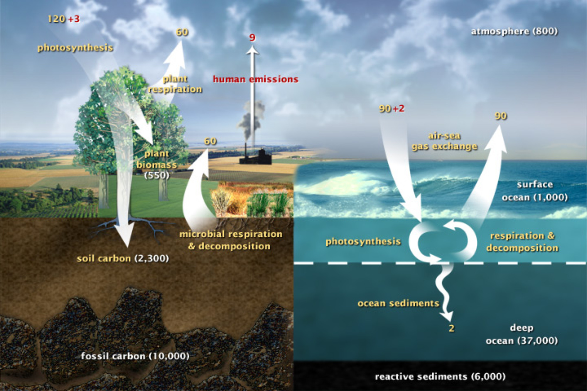
Figure 1: The Carbon Cycle. This diagram of the fast (non-geologic) carbon cycle shows the movement of carbon between land, atmosphere, and oceans. Yellow numbers are natural fluxes, and red are human contributions in gigatons of carbon per year. White numbers indicate stored carbon. Image: NASA Earth Observatory
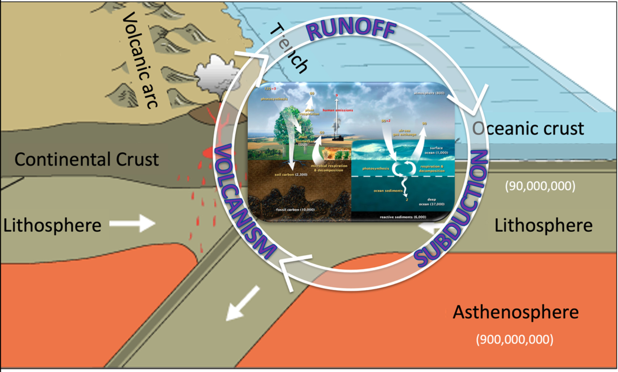
Figure 2: The geologic carbon cycle. The terrestrial and marine carbon cycles from Figure 1, above, are placed within the plate tectonic setting of the geologic carbon cycle. Geologic processes are slower, but move many more gigatons tons of carbon (units are the same as above). Figure by Alexandra Moore for PRI's Earth@Home project (CC BY-NC-SA 4.0 license)
C-Cycle Fluxes: Data Collection
The first step of this experiment is to make the one-liter CO₂ flux chambers. This requires collecting empty plastic bottles ahead of time to have enough for your class. There is a separate YouTube video that takes you and your students step-by-step through the process of cutting up the bottles to make the chambers.
Video: "In the Greenhouse #11 | How to Make a CO2 Flux Chamber" by Alexandra Moore for PRI (YouTube)
In brief, this experiment involves placing a CO₂ probe into the plastic flux chamber, then placing the chamber over a small patch (or pot) of soil, and monitoring the CO₂ concentration in the chamber for a period of appx. 10 minutes. When you initially set up the CO₂ probes for the activity, conduct all your usual pre-lab checks to make sure everything is working and/or whether the probes need to be calibrated. With most CO₂ probes you will find that they need to “settle down” a little after you turn them on and before you use them. Note that if you re-run this experiment with the same flux chamber bottles your students will need to make sure that any accumulated CO₂ is dispersed between experimental runs. Waving the empty bottles around for a minute is a good way to do this. An important aspect of the experimental set-up is that the CO₂ probes fit loosely in the top of the bottle, allowing gas to pass through and out of the system.
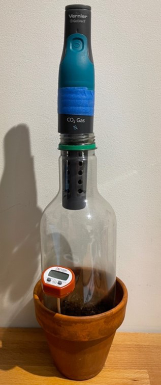
Figure 3: Flowerpot with flux chamber, CO₂ probe, and optional soil thermometer.
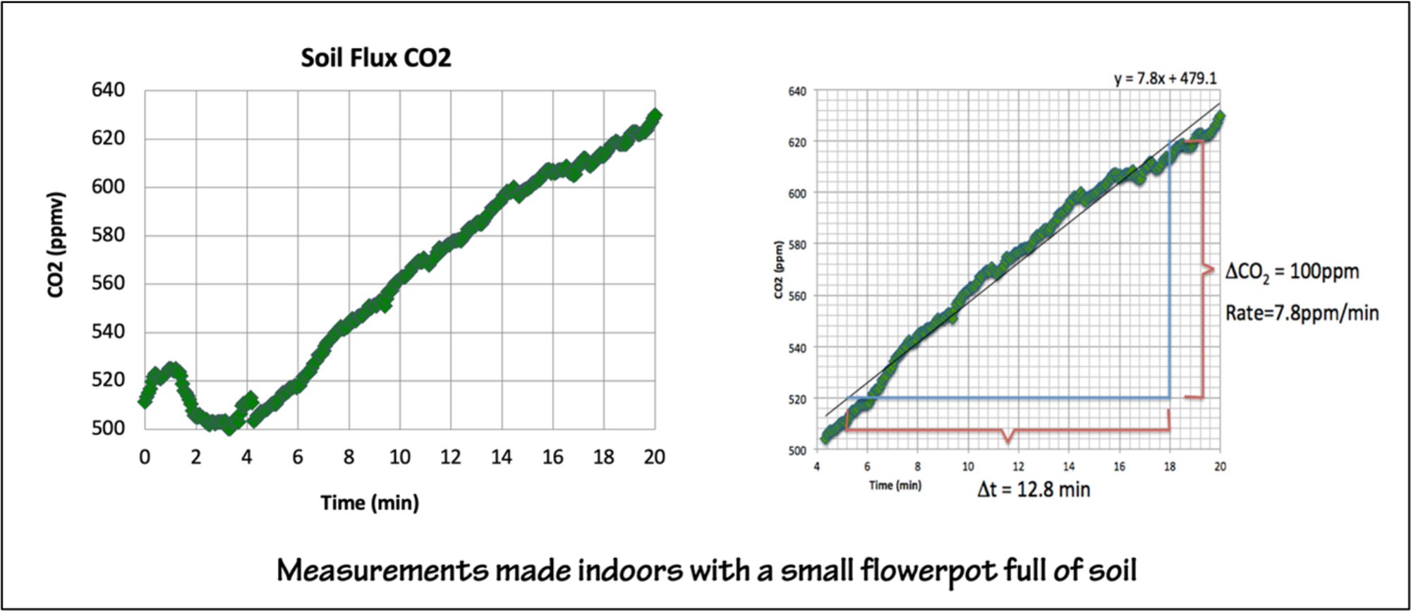
Figure 4: Sample data from an indoor experiment, where the CO2 flux will typically be low. Figure by Alexandra Moore for PRI's Earth@Home project (CC BY-NC-SA 4.0 license)
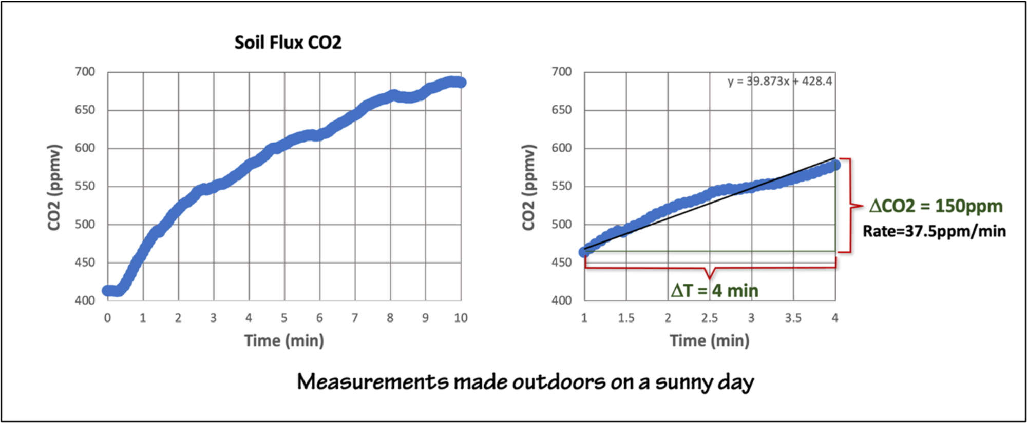
Figure 5: Sample data from an outdoor experiment. Here the CO2 flux is larger so we run the experiment for a shorter period of time. Figure by Alexandra Moore for PRI's Earth@Home project (CC BY-NC-SA 4.0 license)
Graphing & Analysis
Students should plot their measured concentrations as a time series, either by hand or using any graphing software. Based on the behavior of their particular experiment, students can then select a time segment to calculate the slope of a straight-line fit to their data. The slope of the line is the rate of change of CO₂ concentration due to soil respiration:
ΔCO₂ (ppmv) / ΔTime (min) = Flux (ppmv/min)
The data collected by the CO2 probe is in units of concentration – parts per million. It is often more useful to work in units of mass: grams, kilograms or metric tons of CO2. If students compare their own measurements to those published in the literature they will have to do some unit conversion. For example, in Figure 1 the fluxes are given as gigatons of carbon per year. In the Unit Conversion Chart below we will convert the measured concentration change into a mass flux of CO2 – the mass of CO2 per unit volume per unit time. We will use metric (mks) units, so we should end up with kg/s (or kg/min).
Flux is an extensive property; one that changes with the size of the system. For example, the longer we observe, the more CO2 moves through the flux chamber, or, the larger the chamber the more CO2 will move through it. Therefore, we need to normalize our measurement with respect to both time and the cross-sectional area of the flux chamber. The rate calculation already accounts for the time of observation. We still need to account for the basal area of the flux chamber.
Units in Atmospheric Chemistry
Units and unit conversion are often tricky and always important. Also tricky is the fact that the units used in atmospheric chemistry might be unfamiliar to students.
Carbon dioxide is a trace gas in the atmosphere and its concentration is most commonly measured in parts per million by volume (ppmv). The current concentration of atmospheric CO2 is 420 ppmv. Every million molecules of air contain 420 molecules of CO2. In contrast, carbon dioxide emissions are usually reported in gigatons (Gt) = one billion metric tons (1 metric ton = 1000 kg). A gigaton is also a petagram (Pg): 1015 grams. In order to convert units from concentration (ppmv) to mass (kg) students will first need to convert their measured volume to moles of CO2 gas, and then convert moles to kilograms.
➔ An important note: atmospheric chemistry differs from aquatic chemistry, where a concentration of 1 ppm = 1 mg/liter. Because gases can easily expand in volume, this relationship is not true for gas concentrations in the atmosphere. This is why we specify ppmv, and why we have to first convert gases to moles in order to find mass.
Table 1: Unit Conversion from Concentration to Mass Flux of CO2
Steps in Unit Conversion
Result
- Calculate the cross-sectional area of the flux chamber in units of square meters.
m²
- Recall that at standard temperature and pressure (STP) one mole of gas occupies a volume of 22.4 liters. Invert this quantity to find the number of moles in a single liter of gas (e.g. the size of our flux chamber).
mol
- From the graphed data, calculate the rate of change of CO2 in the flask in ppmv/second.
ppmv/s
- Convert this rate of change from ppmv to its decimal equivalent (to do this, divide the rate by 1,000,000). This allows us to use the rate to calculate mass.
- Multiply the rate from Step 4 by the number of moles from Step 2, then divide by the cross-sectional area of the flux chamber from Step 1. The result is the flux of CO2 in units of mol/m2/s.
mol/m²/s
- The mass of CO2 is 44 g/mol (C=12, O=16). Multiply the result from Step 5 by 44 g/mol to convert the flux to units of g/m2/s.
gCO₂/m²/s
- This result is what we were looking for: the mass flux of CO2 per unit area per unit time. In order to compare our result with published data, there are most likely more unit conversions to do—but simpler ones—converting g to kg or minutes to years. See below.
CO₂ Experiments Indoors and Outdoors
The simplest version of this experiment—one flux chamber on a patch of bare soil—is the same in both indoor and outdoor environments. But each setting offers different opportunities to ask additional questions. For example, working indoors with small flower pots allows students to manipulate some of the environmental parameters that control respiration, like temperature and moisture. Working outdoors, students can investigate the balance between photosynthesis and respiration.
Tips & Tricks
Two important aspects of conducting respiration experiments:
- Student-grade CO₂ gas probes can be somewhat fussy instruments
- Soil respiration is heterogeneous, both in a natural outdoor environment and when using potting soil indoors
For both of these reasons, if students conduct paired experiments, it is important to hold constant as many variables as possible. Let the CO₂ probes sit still and equilibrate with the ambient environment for 5-10 minutes before beginning an experiment. Make measurements as closely-spaced in time as possible (e.g. don't conduct the measurements on two separate days). If using flowerpots, use the same soil sample and CO₂ probe for each of the heating and chilling experiments.
Don't let students breathe on the probes (until after they're done) and for the same reason they shouldn't hover over the apparatus while the probe is measuring CO₂ flux. When working outdoors, wind can significantly disturb the CO₂ concentration in the flux chamber. Use a sweater or jacket to shield the chambers on a windy day.
When you do the experiment the magnitude and rate of change will vary depending on your local conditions and whether you are running the experiment outdoors or indoors. An amenable environment for respiration will produce better results, for example, the soil shouldn’t be too cold, too wet, or too dry. If you want the students to graph the results by hand, make the sampling interval long enough that they are not overwhelmed with data, ex. at 15-second intervals for 3-4 minutes. The rates in Figures 4 & 5 are typical.
When working with gases students need to understand the concept of the mole as a unit of molecular mass. The units that a laboratory CO₂ gas probe measures – parts per million – are parts per million by volume (ppmv), rather than the parts per million by mass that is common in aquatic chemistry. In order to convert measurements made in units of ppmv to mass units like grams of carbon, students will need to first convert ppmv to moles of gas, then moles to grams of gas. For middle school students, or others who have not yet encountered moles as units of molecular mass, the simple rate calculation can substitute for the mass flux in most situations, and can be used to compare the behavior of different systems.
Links
Indoor Experiment
Prepare enough soil for your class. If you are using commercial potting soil you will need to inoculate it with soil fungi/microbes, as potting soil is sterilized. You can mix in some soil from outside, or add any kind of decomposing organic matter, or a fermented food like yogurt or kombucha. Keep the soil warm and moist to support its biological community ahead of your experiment. Mix your soil sample as well as you can. Soil is very heterogeneous, and your students will get more consistent results is the soil samples are as homogenous as possible. Set up and run the experiment following the instructions in the handout.
The relationship between temperature and respiration
You can run a simple experiment with a single chamber—or—you can investigate how temperature controls soil respiration rate. The data below are for two side-by-side pots of soil, one in an ice water bath, one in a hot water bath. Note that you will need a container without drainage holes if you use a water bath to control the temperature, as flooding the soil will also change the respiration rate.
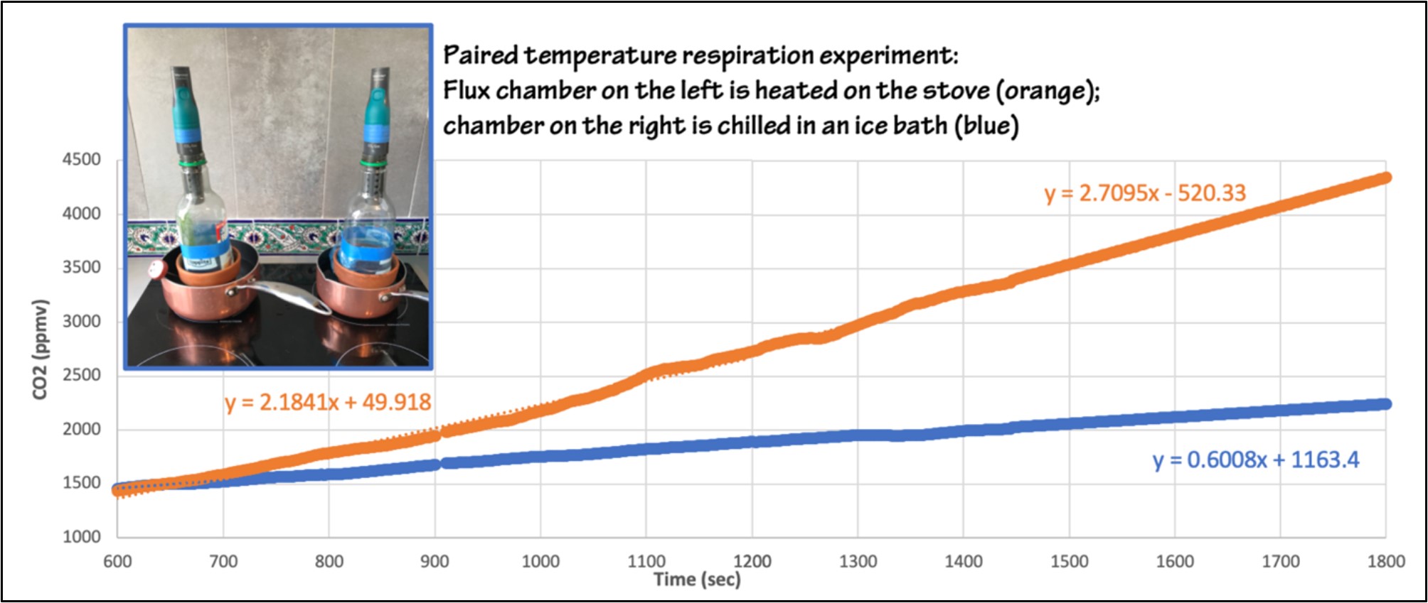
Figure 6: Paired soil respiration experiment. Sample #1 (orange) is heated on the stove, Sample #2 (blue) is chilled in an ice water bath. The graphs show two 30-minute experiments. The slope of the line in the warmed soil experiment increases with increasing temperature, indicating increasing respiration rate as the soil warms. After 30 minutes the CO2 concentration in the heated chamber is approximately double the concentration in the chilled chamber. Figure by Alexandra Moore for PRI's Earth@Home project (CC BY-NC-SA 4.0 license)
A second way to examine the role of changing temperature on soil respiration rate is to use a single experimental set-up that begins chilled, and then warms up (Figure 7). If the soil samples can be stored in a fridge overnight, students can measure the initial respiration rate when they are removed from the fridge, then gradually warm the pots on the stove to monitor the changing respiration. This procedure has the advantage of working with a single system, instead of assuming that the two systems in Figure 6 would behave identically under identical conditions.
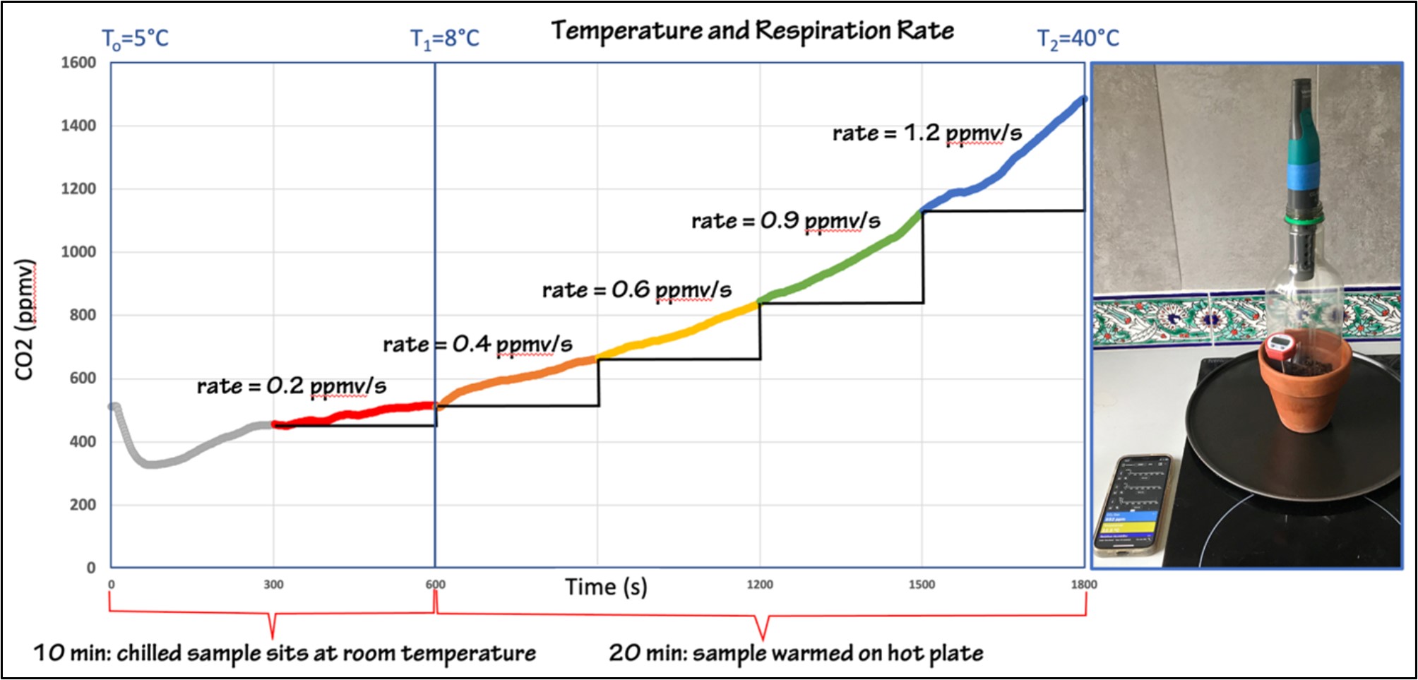
Figure 7: A 30-minute experiment where a chilled soil sample is removed from the refrigerator and allowed to sit at room temp for 10 minutes while CO2 concentration is measured. A soil thermometer in the pot records the change in temperature over this interval, from 5C - 8C. The sample is them warmed on a hot plate for 20 minutes, increasing the soil temperature to 40C. The slope is calculated in 5-minute increments, showing the increasing respiration rate with increasing temperature. In this experiment the first 5 minutes of CO2 data are noisy, and thus not used in the rate comparison. Figure by Alexandra Moore for PRI's Earth@Home project (CC BY-NC-SA 4.0 license)
Outdoors: Conducting a Paired Experiment with opaque and clear flux chambers
An example of the outdoor experiment is shown in the video, "Respiration: Reuse, Recycle"
Video: "Respiration: Reuse, Recycle | In the Greenhouse #12" by Alexandra Moore for PRI (YouTube)
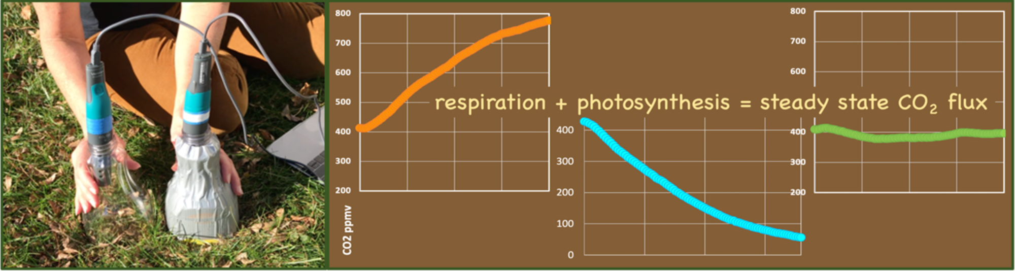
On a grassy outdoor site such as the one shown in the video both photosynthesis and respiration contribute to the CO₂ flux. For this reason, we run a paired experiment with an opaque chamber and a clear chamber. The darkness of the opaque chamber suppresses the photosynthesis of the grass, allowing students to measure the respiration flux. The magnitude of that difference can be seen by conducting the same experiment in the adjacent clear chamber (Figures 8 & 9).
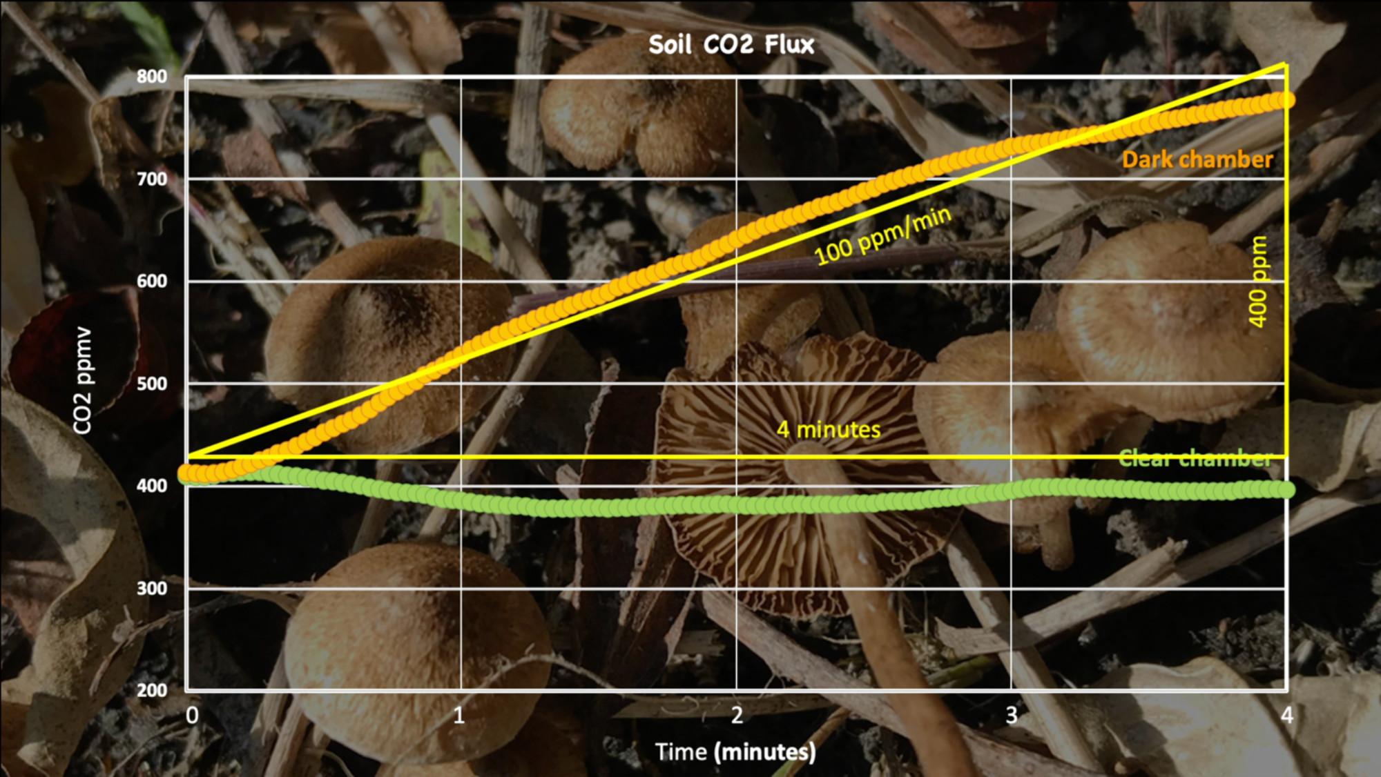
Figure 8: Data from a paired soil CO2 flux experiment with side-by-side opaque and transparent chambers (see discussion of the paired flux experiment below). The flux in the dark chamber, 100ppm/min, is very high--these data were collected on a warm mid-summer day, in an environment with lots of soil organic matter. Figure by Alexandra Moore for PRI's Earth@Home project (CC BY-NC-SA 4.0 license)
Figure 8 above is a typical result for an outdoor measurement in a grassy field on a warm, sunny day. The different results in the clear chamber and the dark chamber each provide for interesting analysis and discussion.
- The dark chamber data are the result of active soil respiration. Students can either use the software that supports the CO₂ probe to find a linear best fit to the data, or can draw a straight line by hand through the data points. The slope of the line gives the rate of CO₂ flux in units of ppm/minute (or ppm/sec if the experiment was set up with x-axis units of seconds).
- The clear chamber is even more interesting. Everything about the two experiments (clear and opaque) is the same —except—that the clear chamber transmits sunlight. Here the grass is photosynthesizing, thus consuming the CO₂ that the soil respires. The sum of these two processes is no significant change in the CO₂ in the chamber.
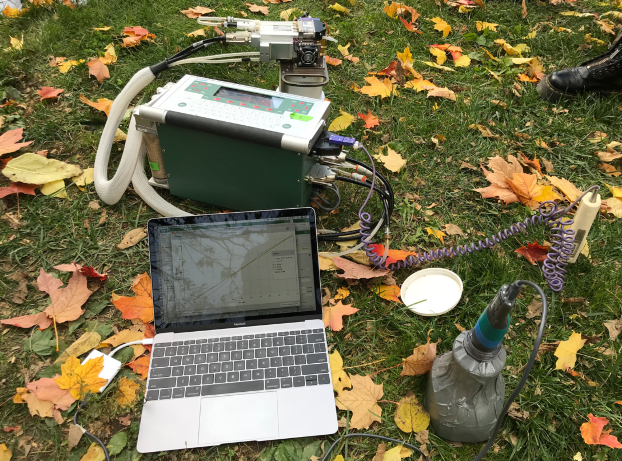
The advantage of conducting this experiment outdoors is that students are measuring an actual environmental flux. When designing this experiment we collaborated with colleagues at Cornell University, and calibrated the measurements made with our Vernier Go-Direct CO₂ probe and plastic bottle flux chamber to data collected with a research-grade LiCOR 6400 CO₂ flux system. The student results were identical to the research-grade data. This result gives us confidence that interesting and powerful observations can be made with very simple tools.
Figure 10: A research-grade LiCOR 6400 CO₂ flux system (top center) is used to calibrate the results of the student experiment (lower right). Photo by Alexandra Moore.
When students quantify their observations they are then able to compare the data that they collect themselves with other local, regional, and global data sets. For this experiment we designed the gas flux chamber to have a volume of one liter. Additionally, we measured the cross-sectional area of the chamber so that we know the area of the soil that we are sampling. These two parameters allow us to convert the units of the student-collected data and compare them with published data for soil CO₂ flux.
Take it Beyond the Classroom
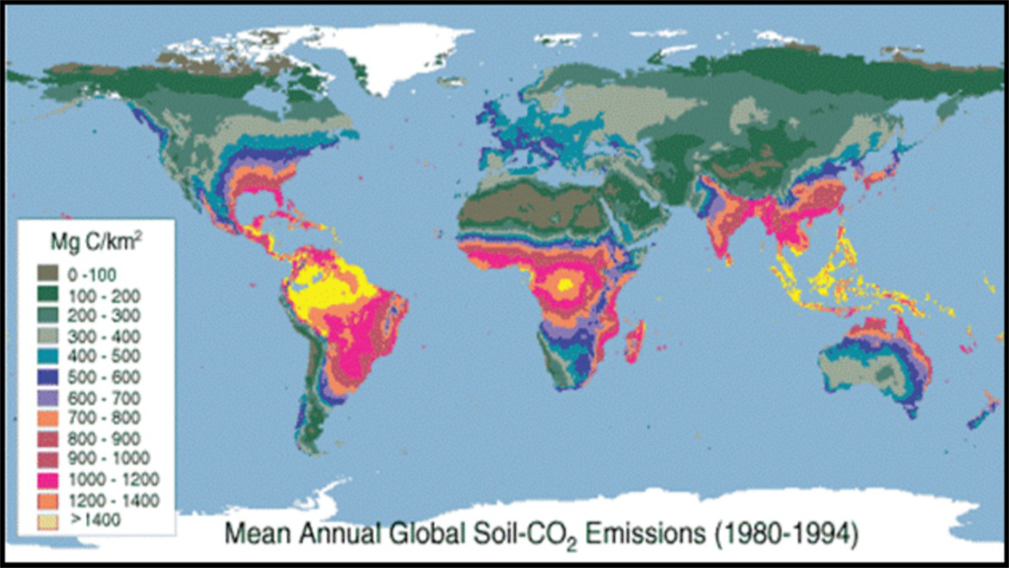
Figure 11: Global mean annual soil carbon flux (MgC/km2/yr), Raich et al., 2003. Figure from Carbon Dioxide Information Analysis Center., U.S. Department of Energy Lawrence Berkeley National Laboratory.
The map above (Figure 11) shows the global variation in annual soil CO₂ flux in units of megagrams (106 grams = 1000 kg = 1 metric ton ) of carbon per square kilometer. In order for students to compare their own data to the global map here they will need to do a multi-step unit conversion. The table below (Table 2) walks students through this process step-by-step. Alternately, you can download an Excel spreadsheet that automates the unit conversion process.
Download Excel unit conversion spreadsheet (780 kB)
Table 2: Additional Unit Conversion
Steps in Unit Conversion
Result
- First change grams of CO2 to grams of carbon. The fraction of C in CO2 is 12/44 (mass of CO2=44, mass of C=12). Multiply your result in Step 6 by (12/44).
gC/m2/s
- Convert the time from seconds to years.
1yr=(365days)(24hrs)(60min)(60sec).
gC/m2/yr
- Convert m2 to km2 (1km=1000m)
gC/km2/yr
11. Convert g to Mg (1Mg=1,000,000g)
MgC/km2/yr
If students can conduct the indoor temperature-control experiments in addition to the outdoor experiment then they will have experience both with the effects of photosynthesis as well as temperature. Even without doing the direct temperature experiments the influence of temperature on respiration rate can be inferred from the global flux map. On the handout we suggest asking questions such as -
- How does your result compare? Is it the same/higher/lower?
- Since the map shows annual values, how might your result be different if you could make measurements all year long?
- Examine the map. Where are C fluxes high (generally)? Where are they low?
- What conclusions can you draw about how environmental conditions control the rates of soil respiration and decomposition?
- If climate is warming globally, how might that change these results several decades into the future?
- Look again at the global carbon cycle in Figure 1. Consider the three terrestrial reservoirs for carbon:
- Atmosphere 800 Gt
- Biosphere 550 Gt
- Soil 2300 Gt
Beyond that, these experiments have implications for the global carbon cycle, and particularly for our climate as the Earth warms. The terrestrial soil carbon reservoir is much larger that the carbon reservoir of terrestrial biomass and that atmospheric carbon reservoir. Increased global temperatures lead to increased soil respiration rates that will transfer carbon from soil to the atmosphere. This is an example of a "positive" or reinforcing feedback. Warmer temperatures lead to faster transfer of CO2 from soil to the atmosphere, where it causes increased warming, which reinforces the faster respiration, etc. The fact that the soil reservoir is almost three times as large as the atmosphere means that the effect of this feedback is potentially very large.
If this conclusion is a source of anxiety for students, encourage them to think about photosynthesis (especially if they have done the paired outdoor experiment) and how simple actions like planting trees actually can have a real impact on climate.
Note about soil respiration map: as of March 2023, the website that hosts these data has been moved here – https://data.ess-dive.lbl.gov/view/doi:10.3334/CDIAC/LUE.NDP081 .Unfortunately, this is a much less user-friendly site than the original – https://cdiac.ess-dive.lbl.gov/epubs/ndp/ndp081/map_yrmn.html. As long as the original site remains on-line, it’s a better resource.